A* search is a fundamental topic in Artificial Intelligence. In this article, let’s see how we can implement this marvelous algorithm in parallel on Graphics Processing Unit (GPU).

Traditional A* Search
Classical A* search implementations typically use two lists, the open list, and the closed list, to store the states during expansion. The closed list stores all of the visited states and is used to prevent the same state from being expanded multiple times. To detect duplicated nodes, this list is frequently implemented by a linked hash table. The open list normally contains states whose successors have not yet been thoroughly investigated. The open list’s data structure is a priority queue, which is typically implemented by a binary heap. The open list of states is sorted using the heuristic function f(x):
f(x) = g(x) + h(x). The distance or cost from the starting node to the current state x is defined by the function g(x), and the estimated distance or cost from the current state x to the end node is defined by the function h(x). The f value is the function value of f(x). When the f values of an issue are small integers, the open list can be efficiently implemented with buckets ¹.
We extract the state with the lowest f value from the open list in each round of A* search, expand its outer neighbors, and check for duplication. The step of detecting node duplication is not required for A* tree search. Following that, we compute the heuristic functions of the resulting states and return them to the open list. If some states’ nodes are already in the open list, we only update their f values for the open list.
In A* search, the heuristic function must be admissible for optimality, which means that h(x) must never be greater than the actual cost or distance to the end node. If the search graph is not a tree, a stronger condition is known as consistency: h(x) ≤ d(x, y) + h(y), where d(x, y) represents the cost or distance from x to y, ensures that once a state is retrieved from the queue, the path it takes is optimal.
Parallel A* Algorithm
Parallelized Computation of Heuristic Functions
In some A* search applications, determining the heuristic functions is very costly and becomes the bottleneck of the entire algorithm. The first step in parallelizing A* search on a GPU in these applications is to parallelize the computation of heuristic functions. This step is simple, and the reasoning is based on the observation that the computation of heuristic functions for each expanded state is mutually independent.
Example for such application
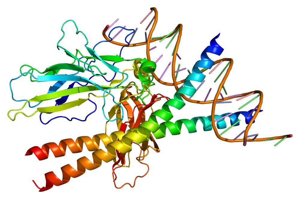
Protein design is a significant problem in computational biology that can be formulated as determining the most likely explanation of a graphical model with a complete graph. To address this issue, A* tree search was created ².
 |
Parallel Priority Queues
After incorporating the preceding procedure, we obtain a simple parallel algorithm. However, on the GPU computational framework, this A* algorithm is still inefficient. Here are the two issues. First, the degree of parallelism is constrained by the outer degree of each node in the search graph. A GPU processor typically has thousands of cores. However, in some applications, such as pathfinding in a grid graph, the degree of a node is typically less than ten, limiting the degree of parallelism on a GPU platform. Second, many sequential parts of this simple algorithm have yet to be fully parallelized.
For example, using a binary heap, the EXTRACT, and PUSH-BACK operations for the open list take O(log N) time to complete, where N is the total number of elements in the list. Priority queue functions will become the most time-consuming parts of A* search in applications where the computation of heuristic functions is relatively cheap. Sequential operations are inefficient for a GPU processor because they only use a small portion of the GPU hardware, and a GPU’s single-thread performance is far inferior to that of a CPU.
To increase the degree of parallelism in the computation of heuristic functions, the first problem can be solved by extracting multiple states from the priority queue. Priority queue operations, on the other hand, continue to operate in a sequential mode. The second problem could be solved by using a concurrent data structure for the priority queue. Existing lock-free concurrent priority queues, such as those proposed in ³, cannot run efficiently on a modern GPU processor’s Single Instruction and Multiple Data Stream (SIMD) architecture because they require the use of compare-and-swap (CAS) operations.
To address both issues, we can create a parallel A* algorithm that takes advantage of the GPU hardware’s parallelism. Instead of using a single priority queue for the open list, we can allocate a large number (typically thousands) of priority queues during A* search. We can extract multiple states from individual priority queues each time, which parallelizes the sequential portion of the original algorithm. This can also boost the number of expanding states at each step, improving the degree of parallelism for the computation of heuristic functions, as discussed previously.
 |
| Image by Author: Data flow of the open list |
Algorithm
We can increase the degree of parallelism by assigning more priority queues (i.e., increasing the parameter k) to further utilize the computational power of the GPU hardware. However, we cannot indefinitely increase the degree of parallelism because extracting multiple states in parallel instead of a single state with the best f value so far can result in overhead on the number of expanded states. The higher the degree of parallelism, the more states Parallel A* must generate in order to find the optimal path. To utilize the computational power of the GPU hardware, we must balance the trade-off between the overhead of extra expanded states and the degree of parallelism.
Node Duplication Detection on a GPU
In A* graph search, we may attempt to expand a state whose node has already been visited. If the new state’s f value is not less than the f value of the existing state in the closed list, it is safe to prevent this state from being visited again. This is known as node duplication detection. The difficulty of detecting node duplication varies depending on the application. This step is not required in the A* tree search. To perform an A* graph search in which the entire graph fits into memory, we can simply use an array table.
The detection of node duplication necessitates the use of a data structure that can support both INSERT and QUERY operations. The INSERT command adds a key-value pair to the data structure. QUERY determines whether or not a key exists in this data structure. If this is the case, it returns the value associated with it. We frequently use a linked hash table or a balanced binary search tree on a CPU platform (such as a red-black tree). However, extending these data structures to parallel node duplication detection on a GPU is extremely difficult. In a linked hash table, for example, it will be difficult to handle the situation in which two different states are inserted into the same bucket at the same time.
So we need to resort to a more appropriate data structure for efficient node duplication detection on a GPU such as,
- Parallel cuckoo hashing, which is a parallelized version of the traditional cuckoo hashing algorithm ⁴.
- Parallel hashing with replacement, which is a probabilistic data structure particularly designed for simplicity on a GPU.
I hope you’ve now understood the way we can have a Parallel Version of the A* Algorithm that can be executed on GPU.
Think about the bidirectional version of this algorithm and try to change the algorithm that can be used to execute this approach bidirectionally.
 |
Will it save more time? Try and find.
Hope this can help. Share your thoughts too.
References
- Dial, Robert. (1969). Algorithm 360: Shortest-path forest with topological ordering [H]. Commun. ACM. 12. 632–633. 10.1145/363269.363610.
- Leach, A. R., and Lemon, A. P. 1998. Exploring the Conformational Space of Protein Side Chains Using Dead-end Elimination and the A* Algorithm. Proteins Structure Function and Genetics 33(2):227–239.
- Sundell, H., and Tsigas, P. 2003. Fast and Lock-free Concurrent Priority Queues For Multi-thread Systems. In Parallel and Distributed Processing Symposium, 2003. Proceedings. International, 11–pp. IEEE.
- Pagh, R., and Rodler, F. F. 2001. Cuckoo Hashing. Springer.
Comments
Post a Comment