Multiclass Classification Using Support Vector Machines

Binary Classification

The machine should only categorize an instance as one of two classes of this type: yes/no, 1/0, or true/false.

In this sort of categorization inquiry, the answer is always yes or no. Is there a human in this photograph, for example? Is there a good tone to this text? Will the price of a specific stock rise in the coming month?

Multiclass Classification

In this case, the machine must categorize an instance into only one of three or more classes. Multiclass categorization may be shown in the following examples:

1. Positive, negative, or neutral classification of a text
2. Identifying a dog breed from a photograph
3. A news item might be classified as sports, politics, economics, or social issue.

Support Vector Machines (SVM)

SVM is a supervised machine learning method that may be used to aid with both classification and regression problems. It aims to determine the best border (hyperplane) between distinct classes. In basic terms, SVM performs complicated data modifications based on the kernel function specified, with the goal of maximizing the partition boundaries across your data points.

SVM aims to identify a line that optimizes the separation between a two-class data set of 2-dimensional space points in its simplest form, where there is a linear separation.

The goal of SVM is to identify a hyperplane in an n-dimensional space that optimizes the separation of data points from their actual classes. Support Vectors are data points that are the shortest distance from the hyperplane, i.e. the nearest points.

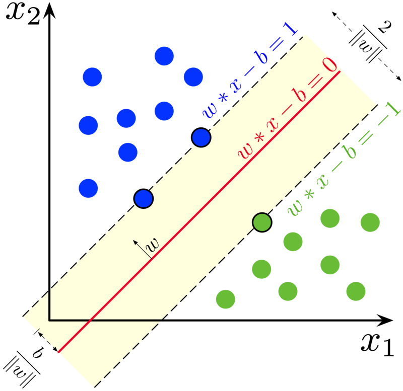
The Support Vectors (2 blue and 1 green) are the three points overlaid on the dispersed lines in the preceding figure, and the separation hyperplane is the solid red line.

SVM-based Multiclass Classification

SVM does not allow multiclass classification in its most basic form. After breaking down the multi-classification problem into smaller subproblems, all of which are binary classification problems, the same technique is used for multiclass classification.

The following are some of the most common ways for doing multi-classification on issue statements using SVM:

1. One vs One (OVO) approach
2. One vs All (OVA) approach
3. Directed Acyclic Graph (DAG) approach
4. Unbalanced Decision Tree (UDT) approach

Let’s take a closer look at each of these techniques one at a time.

One vs One (OVO) approach

This method divides our multiclass classification issue into subproblems, each of which is a binary classification problem. As a result of this technique, binary classifiers for each pair of classes are produced. Use the idea of majority voting, together with the distance from the margin as the confidence criteria, to make a final forecast for any input.

Example: Suppose if we have 4 elements [1, 2, 3, 4]

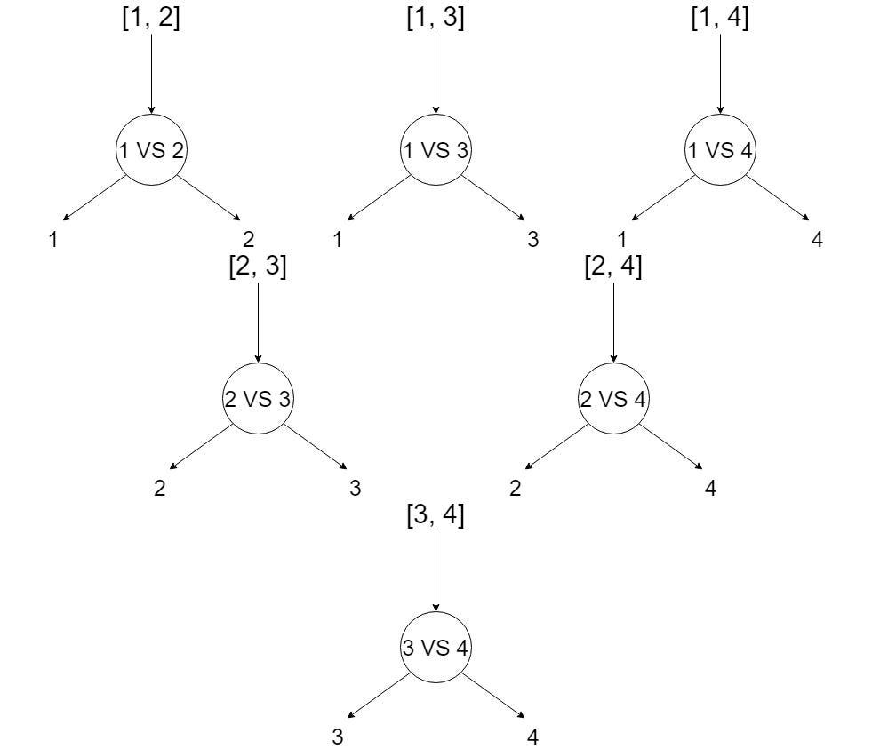
The main issue with this method is that it requires us to train an excessive number of SVMs. For every pair of distinct classes, in total, it constructs 0.5N(N-1) binary classifiers (same number of classifiers for testing and training) where N is the number of classes. The binary classifier Cij is trained with examples from the ith class and jth class only, where examples from Class i take positive labels while examples from Class j generally take negative labels.

For example, if classifier Cij predicts x is in Class i, then the vote for Class i is increased by 1, otherwise, the vote for Class j is increased by 1. The max-wins strategy then assigns x to the Class receiving the highest score.

One vs All (OVA) approach

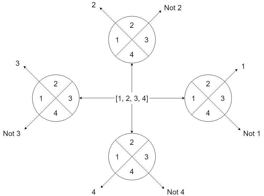
One vs. all is a method of using binary categorization. A-One vs All solution consists of N independent binary classifiers; one binary classifier for each potential outcome for a classification problem with N possible answers. The model is trained by running it through a series of binary classifiers, each of which is trained to answer a different classification question.

That is to say:

• Is this image an orange? No.
• Is this image a dog? No.
• Is this image a cat? Yes.
• Is this image an egg? No.

When the total number of classes is modest, this technique is appropriate, but as the number of classes grows, it becomes increasingly inefficient.

In brief; if we have an N-class issue, we learn N SVMs using this technique:

"class output = 1" vs. "class output 1" is learned by SVM1

"class output = 2" vs. "class output 2" is learned by SVM2

.

.

.

"class output = N" vs. "class output N" is learned by SVMN

Then, to predict the output for fresh input, just predict with each of the built SVMs and see which one places the prediction the furthest into the positive zone (behaves as a confidence criterion for a particular SVM).

There are several difficulties in training these N SVMs, including:

• Excessive Computation

We need additional training points to execute the OVA approach, which increases our computation.

• Problems become imbalanced

Suppose you’re working on an MNIST dataset with ten classes ranging from 0 to 9, and each class has 1000 points. If each SVM has two classes, one will have 9000 points and the other will have just 1000 data points, resulting in an unbalanced problem.

To resolve these issues, you must select a representative (subsample) from the majority class, which has the most training samples. You can accomplish so by employing the following methods:

1. Be using normal distribution’s 3-sigma rule.
2. Take a few data points from the majority class at random.
3. Use SMOTE, a common subsampling method.

Directed Acyclic Graph (DAG) approach

A directed acyclic graph (DAG) is a diagram that depicts a succession of actions. A graph depicting the sequence of the activities is visually shown as a series of circles, each representing an activity, some of which are connected by lines, which reflect the flow from one activity to the next.

This method is more hierarchical in structure, and it attempts to overcome the issues that the One vs One and One vs All methods have. This is a graphical technique in which the classes are grouped according to some logical grouping.

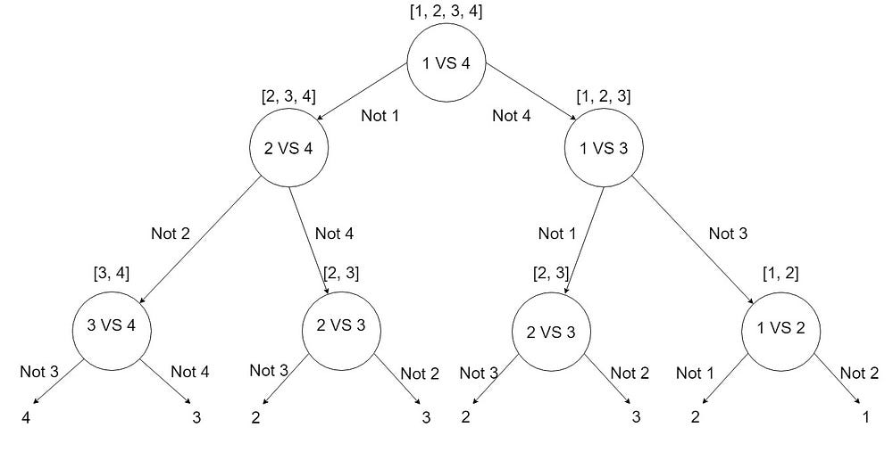
DAG-based SVMs are implemented using a “Leave One Out” method. The Training phase of DAG is the same as that of the OVO method. In the testing phase, it uses a rooted binary directed acyclic graph which has 0.5N(N-1) internal nodes and N leaves. In this example, we have 6 decision nodes and 4 leaves. For testing, we use N-1 classifiers.

How 6 decision nodes? Well, look at this image.

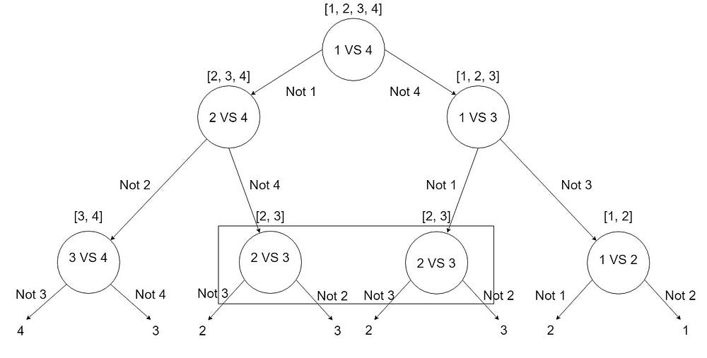
Benefits: When compared to the OVA technique, this approach has fewer SVM trains and reduces the variability from the majority class, which is an issue with the OVA approach.

Problem: If we have given the dataset itself in the form of different groups (e.g., CIFAR-10 image classification dataset), we can apply this approach directly; however, if we haven’t given the groups, the problem with this approach is that we have to manually pick the logical grouping in the dataset.

Unbalanced Decision Tree (UDT) approach

To make a judgment on any input pattern, UDT-based SVMs use a “Knock Down” method using most N-1 classifiers. Each UDT decision node is a best-fit classification model. The OVA-based classifier that gives the highest performance metric is the best model for each decision node.

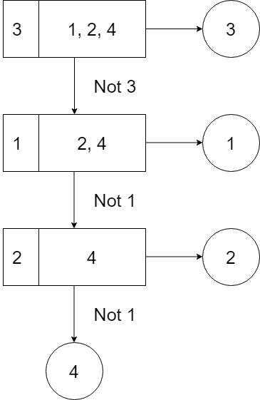
The optimum model compares one selected class to the others, starting at the root node. The UDT then moves on to the next level of the decision tree by removing the selected class from the previous level. The UDT ends when it returns an output pattern at the decision node level, but the DAG must continue until it reaches a leaf node.

Additional tip

There are numerous scenarios that might lead to the use of decision tree models to handle imbalanced issues; you can examine whether the situation you described in your query fits into any of the following categories:

• Minority data are all in one area of the feature space.

The decision tree’s training process is recursive; the algorithm will continue to pick the best partitioning features, as well as the production of branches and nodes until it reaches:

1. The samples in the current node all belong to the same category, therefore there is no need to separate them.
2. The attribute set is empty, or all samples have identical attribute values, making division impossible.
3. The sample-set at the current node is empty, and thus cannot be split.

So, if the minority data are all in one region of the feature space, all samples will be partitioned into a node, and if the test set is likewise in this feature distribution, a decent classifier will be obtained in the prediction.

• You’re employing a decision tree with cost-sensitive learning.

Misclassifications of minority class samples will cost more than misclassifications of majority class samples if your judgment is cost-sensitive.
The model will perform well if you utilize ensemble learning, but it isn’t the decision tree; it’s RF or GBDT.

When presented with an imbalanced situation, basic linear regression classifiers, such as logistic regression, almost definitely perform poorly. This is because, during training, the model looks for a hyperplane with the least amount of misclassification. As a consequence, the model assigns all samples to the most appropriate label.

Hope this helps. Share your thoughts too.